To make reactomics data analysis more transparent and reproducible, I included one template in rmwf package. You could install the package from Github.
install.packages('remotes')
remotes::install_github("yufree/rmwf")
If you use RStudio, you could try:
File-New file-R Markdown-from template
Then select ‘reactomics’ to use template for reactomics analysis. Here is a preview for data analysis of this study:
Demo data
path <- system.file("demodata/untarget", package = "rmwf")
files <- list.files(path,recursive = T,full.names = T)
ST000560pos <- enviGCMS::getmzrtcsv(files[grepl('ST000560mzrt',files)])
Remove the redundant peaks
# check the paired mass distance relationship
pmd <- pmd::getpaired(ST000560pos)
## 56 retention time cluster found.## 826 paired masses found## 23 unique within RT clusters high frequency PMD(s) used for further investigation.## The unique within RT clusters high frequency PMD(s) is(are) 12 2.02 26.02 28.03 14.02 26.01 54.05 24 9.99 40.03 44.04 2.01 15.01 30.01 27.02 44.03 14.01 21.98 30.05 42.05 29.02 4.03 66.02.## 182 isotopologue(s) related paired mass found.## 1145 multi-charger(s) related paired mass found.pmd::plotpaired(pmd)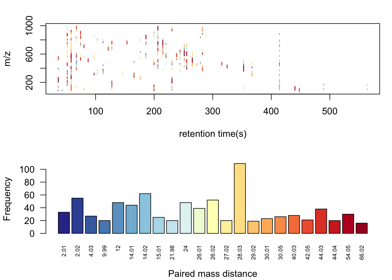
Here we could see some common PMDs within the same retention time bins like 21.98Da for the mass differences between [M+Na] and [M+H]. Other PMDs might refer to in-source reaction such as PMD 2.02Da for opening or forming of double bond. Another common kinds of PMDs should the homologous series compounds which could not be separated by the column such as PMD 14.02Da for CH2, PMD 28.03Da for C2H4, PMD 44.03Da for C3H6, and 56.05Da for C4H8, as well as 58.04Da for C3H6O. There are also some PMDs which highly depended on the the samples’ matrix. Anyway, we will check those high frequency PMD considering isotopes, as well as multiple chargers to extract one peak for one potential compound. Such algorithm is called GlobalStd. The advantage of GlobalStd is that no pre-defined paired mass distances list is needed to remove redundant peaks. When a PMD appeared with high frequency in certain samples, it will be treated as potential adducts to be removed.
std <- pmd::getstd(pmd)## 4 retention group(s) have single peaks. 52 54 55 56## 10 group(s) with multiple peaks while no isotope/paired relationship 26 30 33 35 45 47 48 49 51 53## 2 group(s) with multiple peaks with isotope without paired relationship 29 32## 20 group(s) with paired relationship without isotope 10 11 13 14 15 16 18 20 23 27 28 31 36 38 40 42 43 44 46 50## 20 group(s) with paired relationship and isotope 1 2 3 4 5 6 7 8 9 12 17 19 21 22 24 25 34 37 39 41## 196 std mass found.pmd::plotstd(std)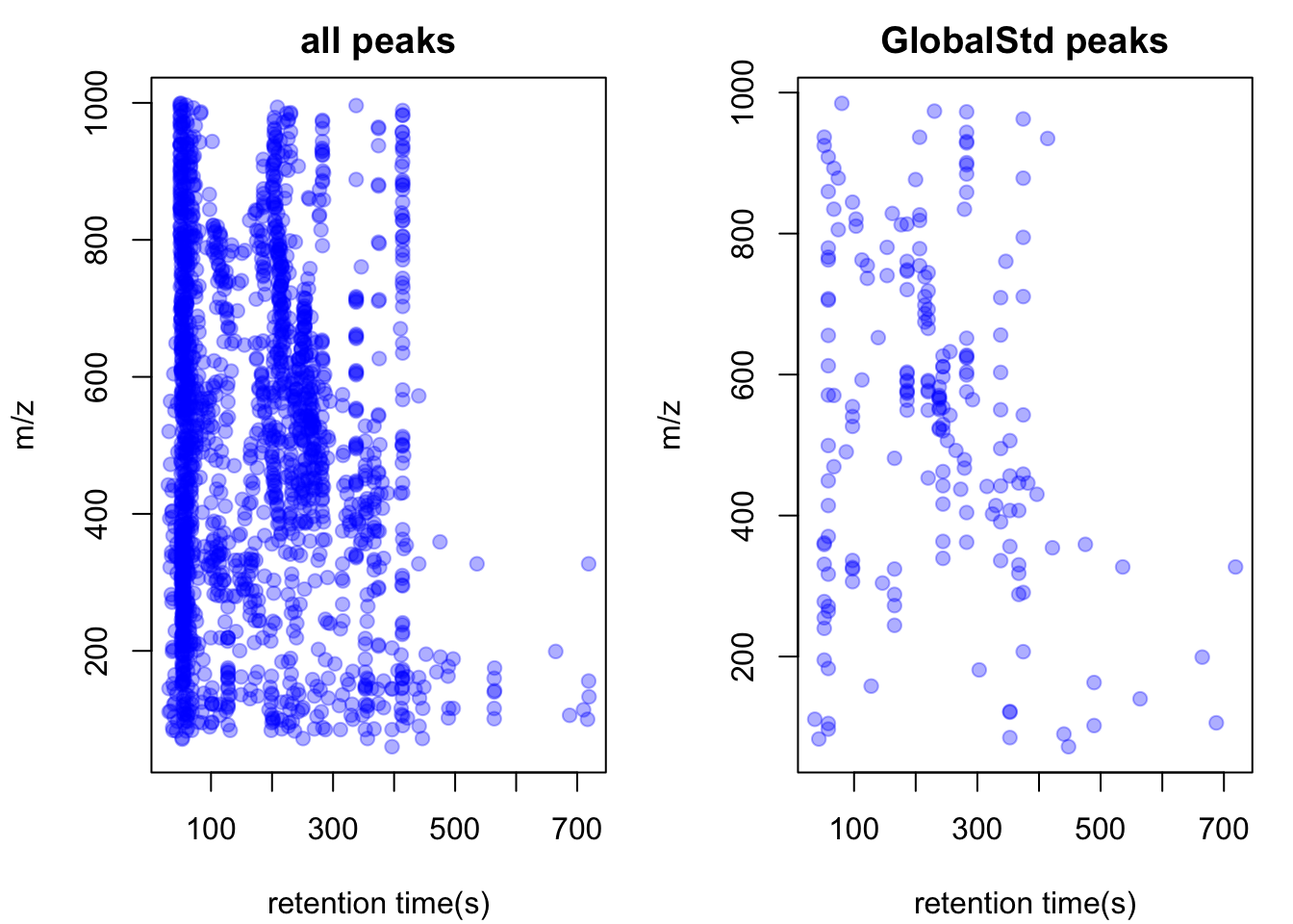
In this case, we get 205 peaks for 205 potential compounds. Now we could retain those peaks for reactomics analysis.
# generate new peak list and matrix sample
peakstd <- enviGCMS::getfilter(std,rowindex = std$stdmassindex)
GlobalStd algorithm was originally designed to retrieve independent peaks by the paired mass distances relationship among features without a predefined adducts or neutral loss list. However, the peaks from the same compounds should also be correlated with each other. Meanwhile, the independent peaks selection might still have peaks from the same compounds when the peaks’ high frequency PMDs are not independent. In this case, the GlobalStd algorithm could set a cutoff to re-check the independent peaks by their relationship with potential PMDs groups and select the base peaks for the clusters of peaks.
Meanwhile, network analysis could be used for PMDDA workflow to select precursor ion for MS/MS annotation. Such precursor ions was selected by checking the peak with highest intensity of each independent peaks’ high frequency PMD network cluster, which could be treated as pseudo spectra.
Extract high frequency PMDs
To retrieve the general chemical relationship, we will focus on high frequency PMDs within a certain metabolic profile. If one PMD occur multiple times among peaks from a snapshot of samples, certain reactions or bio-process should be important or occur multiple times compared with rarely PMD, which could be a random differences among compounds. In this case, extraction of high frequency PMDs will refine the investigation on a few active reactions instead of treating each peak individually, which is almost impossible for untargeted analysis.
Such PMDs frequency analysis should be performed on the data set with the redundant peaks removal. Otherwise, the high frequency PMD among compounds will be immersed by PMD with from isotopes, adducts or other common PMDs from the backgrounds.
You could define the cutoff of frequency while the default setting using the largest PMD network cluster numbers to determine the cutoff, which try to capture more information. Here we will retrieve high frequency PMDs from the demo data using a larger cutoff to reduce the complexity:
hfp <- pmd::getsda(std,freqcutoff = 8)## 8 groups were found as high frequency PMD group.## 0 was found as high frequency PMD.
## 2.02 was found as high frequency PMD.
## 12 was found as high frequency PMD.
## 14.02 was found as high frequency PMD.
## 24 was found as high frequency PMD.
## 26.02 was found as high frequency PMD.
## 28.03 was found as high frequency PMD.
## 50.01 was found as high frequency PMD.pmd::plotstdsda(hfp)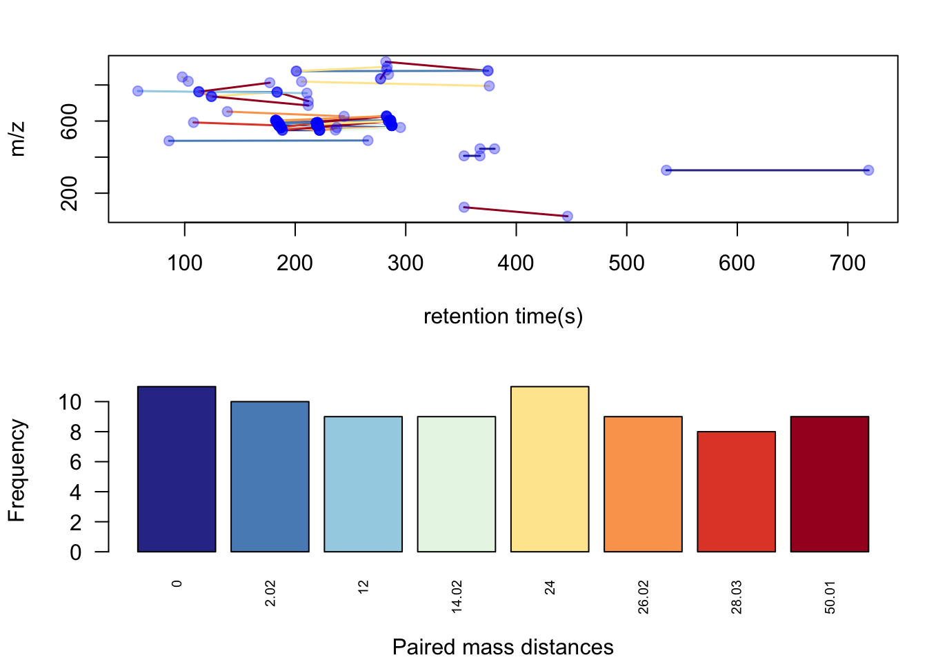
Here we could find 8 PMDs were selected as high frequency PMDs. PMD 0 Da could be some isomers, PMD 2.02 Da could be reduction reactions, etc. Some PMDs can be the combination of other PMDs, which could be a chain reactions. From the plot you might also identify the homologous series by the retention times relations.
When you have the lists of high frequency PMDs, you could check the PMDs changes among groups. Here we will quantitatively analysis certain PMD to show the reaction level changes.
# remove QC sample
hfp2 <- enviGCMS::getfilter(hfp,colindex = !grepl('QC',hfp$group$sample_group))
# check pmd 14.02
qreact <- pmd::getreact(hfp2,pmd = 14.02)
qreactsum <- apply(qreact$data,2,sum)
t.test(qreactsum~qreact$group$sample_group)
##
## Welch Two Sample t-test
##
## data: qreactsum by qreact$group$sample_group
## t = 2.2, df = 17, p-value = 0.04
## alternative hypothesis: true difference in means is not equal to 0
## 95 percent confidence interval:
## 2939 95129
## sample estimates:
## mean in group control mean in group IgAN
## 1247817 1198783par(mfrow=c(1,1))
boxplot(qreactsum~qreact$group$sample_group,xlab='',ylab = 'intensity', main='PMD 14.02Da')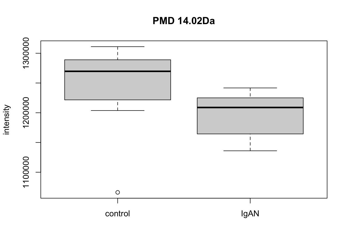
Here we could find PMD 14.02Da could be a biomarker reaction for case and control. Meanwhile, paired relationship could be connected into network to show the overall relationship within the samples.
Reactomics network analysis
The relation among those high frequency PMDs peaks could be further checked in two ways by network analysis: one from the correlation analysis and another from the PMD analysis. If we combined them together, reactomics network could be generated to capture the major reaction network within the samples. We will check them step by step.
Build the correlation network
library(igraph)##
## Attaching package: 'igraph'## The following objects are masked from 'package:stats':
##
## decompose, spectrum## The following object is masked from 'package:base':
##
## unioncutoff <- 0.9
metacor <- stats::cor(t(peakstd$data))
metacor[abs(metacor)<cutoff] <- 0
df <- data.frame(from=rownames(peakstd$data)[which(lower.tri(metacor), arr.ind = T)[, 1]],to=rownames(peakstd$data)[which(lower.tri(metacor), arr.ind = T)[, 2]],cor=metacor[lower.tri(metacor)])
df <- df[abs(df$cor)>0,]
df$direction <- ifelse(df$cor>0,'positive','negative')
net <- igraph::graph_from_data_frame(df,directed = F)
netc <- igraph::components(net)
message(paste(netc$no, 'metabolites correlation network clusters found'))## 16 metabolites correlation network clusters foundindex <- rep(NA,length(rownames(peakstd$data)))
index[match(names(netc$membership),rownames(peakstd$data))] <- netc$membership
message(paste(sum(is.na(index)), 'out of', length(rownames(peakstd$data)), 'metabolites have no correlation with other metabolites'))## 88 out of 197 metabolites have no correlation with other metabolitesplot(net,vertex.label=NA,vertex.size =5,edge.width = 3, main = 'Correlation network')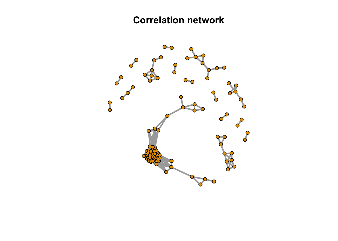
Here we could see the correlation among those peaks as network. 109 peaks have relations with each others and 88 peaks were single.
Build the PMD network
peaksda <- pmd::getsda(std,freqcutoff = 8)## 8 groups were found as high frequency PMD group.## 0 was found as high frequency PMD.
## 2.02 was found as high frequency PMD.
## 12 was found as high frequency PMD.
## 14.02 was found as high frequency PMD.
## 24 was found as high frequency PMD.
## 26.02 was found as high frequency PMD.
## 28.03 was found as high frequency PMD.
## 50.01 was found as high frequency PMD.df <- peaksda$sda
df$from <- paste0('M',round(df$ms1,4),'T',round(df$rt1,1))
df$to <- paste0('M',round(df$ms2,4),'T',round(df$rt2,1))
net <- graph_from_data_frame(df[,c('from','to','diff2')],directed = F)
netc <- igraph::components(net)
message(paste(netc$no, 'metabolites PMD network clusters found'))## 15 metabolites PMD network clusters foundindex <- rep(NA,length(rownames(peakstd$data)))
index[match(names(netc$membership),rownames(peakstd$data))] <- netc$membership
message(paste(sum(is.na(index)), 'out of', length(rownames(peakstd$data)), 'metabolites have no PMD relations with other metabolites'))## 143 out of 197 metabolites have no PMD relations with other metabolitespal <- grDevices::rainbow(8)
plot(net,vertex.label=NA,vertex.size =5,edge.width = 3,edge.color = pal[as.numeric(as.factor(E(net)$diff2))], main = 'PMD network')
legend("topright",bty = "n",
legend=unique(E(net)$diff2),
fill=unique(pal[as.numeric(as.factor(E(net)$diff2))]), border=NA,horiz = F)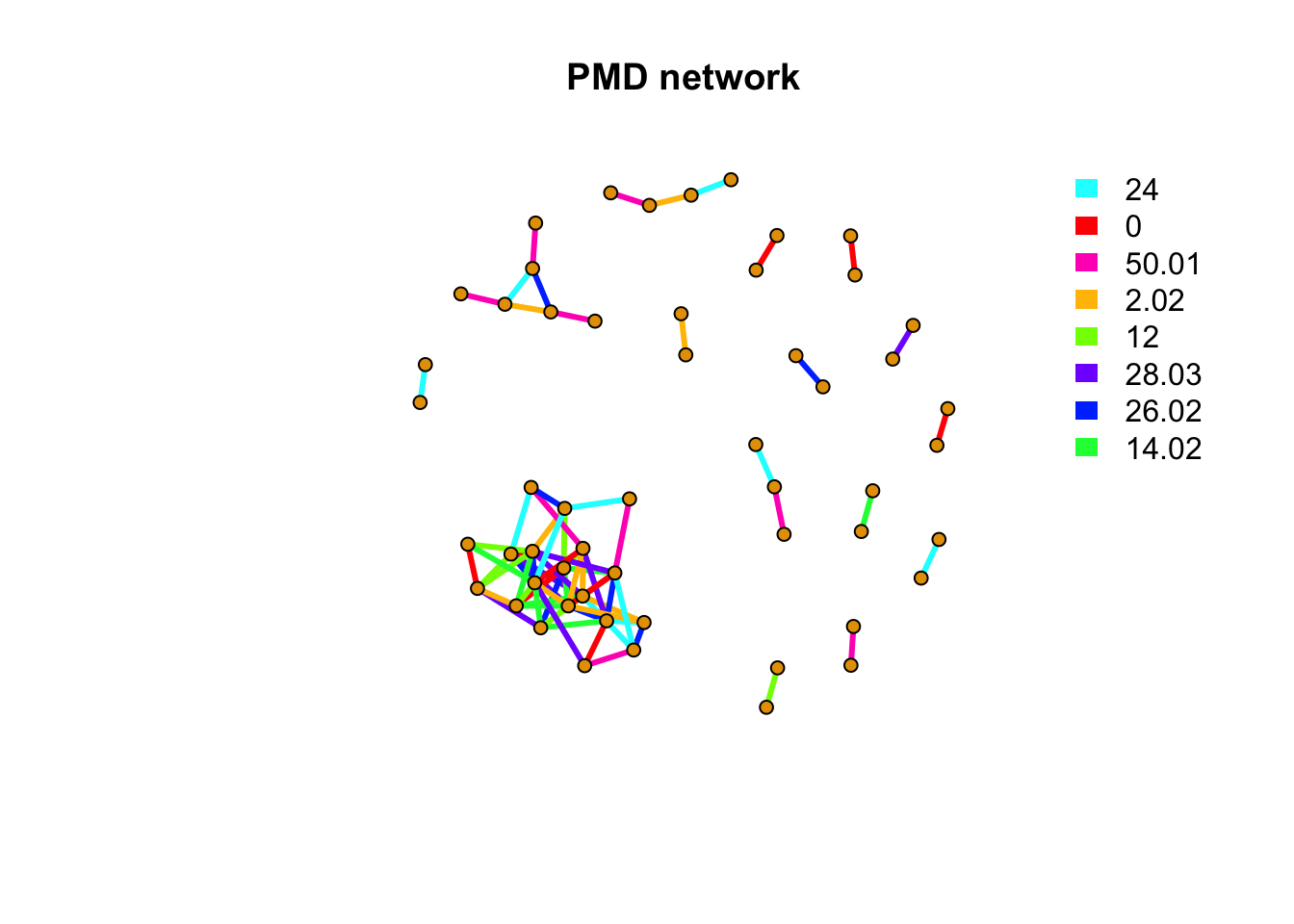
unique(E(net)$diff2)## [1] 24.00 0.00 50.01 2.02 12.00 28.03 26.02 14.02By checking the high frequency PMD relation, we see a similar while different results. Those high frequency PMDs could also be linked to potential reactions such as 0Da for isomers, 2.02Da for double bonds breaking/forming. Such PMDs could reveal the major reactions found among the metabolites. 54 peaks have PMDs relations with each others and 143 peaks were single.
Here we need to define a frequency cutoff. With the increasing number of high frequency PMDs cutoff, the ions cluster numbers would firstly increase then decrease. At the very beginning, the increasing numbers will include more information because high frequency PMDs always capture real reactions or structures relationships among compounds. Low frequency PMDs will introduce limited information as they might be generated by random differences among ions. In terms of network analysis, when the high frequency PMD cutoff is small, the network clusters will be small. However, when the numbers of network clusters are not increasing any more with more PMDs included, the relationship information among ions will not increase and the cutoff could be automated detected by GlobalStd algorithm. In detail, the algorithm will try to include PMDs one by one starting from the highest frequency PMDs. Meanwhile, the ions cluster numbers were recorded for the generated network among independent peaks and the cutoff will be the PMDs list with the largest number of independent peaks’ network cluster.
Build the PMD network with correlation
We could combine the PMD relation with correlation together to show the quantitative reactomics networks within the samples. Those metabolites could be quantitatively checked among different samples.
peaksda <- pmd::getsda(std,freqcutoff = 8,corcutoff = 0.6)## 8 groups were found as high frequency PMD group.## 0 was found as high frequency PMD.
## 2.02 was found as high frequency PMD.
## 12 was found as high frequency PMD.
## 14.02 was found as high frequency PMD.
## 24 was found as high frequency PMD.
## 26.02 was found as high frequency PMD.
## 28.03 was found as high frequency PMD.
## 50.01 was found as high frequency PMD.df <- peaksda$sda
df$from <- paste0('M',round(df$ms1,4),'T',round(df$rt1,1))
df$to <- paste0('M',round(df$ms2,4),'T',round(df$rt2,1))
net <- graph_from_data_frame(df[,c('from','to','diff2')],directed = F)
netc <- igraph::components(net)
message(paste(netc$no, 'metabolites quantitative reactomics network clusters found'))## 10 metabolites quantitative reactomics network clusters foundindex <- rep(NA,length(rownames(peakstd$data)))
index[match(names(netc$membership),rownames(peakstd$data))] <- netc$membership
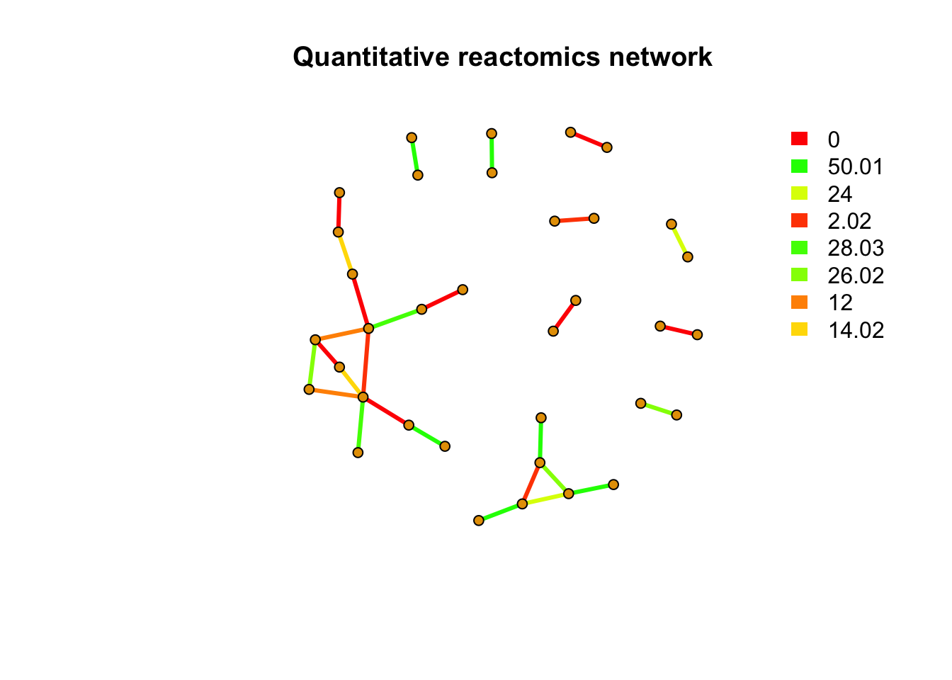
message(paste(sum(is.na(index)), 'out of', length(rownames(peakstd$data)), 'metabolites have no PMD&correlation relations with other metabolites'))## 162 out of 197 metabolites have no PMD&correlation relations with other metabolitesnet <- graph_from_data_frame(peaksda$sda,directed = F)
pal <- grDevices::rainbow(21)
plot(net,vertex.label=NA,vertex.size =5,edge.width = 3,edge.color = pal[as.numeric(as.factor(E(net)$diff2))], main = 'Quantitative reactomics network')
legend("topright",bty = "n",
legend=unique(E(net)$diff2),
fill=unique(pal[as.numeric(as.factor(E(net)$diff2))]), border=NA,horiz = F)