Our HMDB data have 114066 metabolites with 13 properties such as hmdb ID, monisotopic_molecular_weight, iupac_name, name, chemical_formula, cas_registry_number, smiles, kingdom, direct_parent, super_class, class, sub_class, molecular_framework. Let’s make some explore analysis:
Ratio between monisotopic molecular weight and smiles
library(tidyverse)
hmdb %>%
        summarise_all(funs(n_distinct(.)))
## # A tibble: 1 x 13
##   accession monisotopic_molecular_weig… iupac_name   name chemical_formula
##       <int>                       <int>      <int>  <int>            <int>
## 1    114066                       13429     113720 114066            11762
## # ... with 8 more variables: cas_registry_number <int>, smiles <int>,
## #   kingdom <int>, direct_parent <int>, super_class <int>, class <int>,
## #   sub_class <int>, molecular_framework <int>
We have 13429 monisotopic molecular weight, 11762 chemical formula, 113900 smiles among the 114066 metabolites, which means for each monisotopic molecular weight, you could find ~8.5 metabolites. Different smiles means different structures and this is the main reason why we need MS/MS data. However, we could check the ratio in details.
library(tidyverse)
hmdb %>%
        group_by(super_class) %>%
        summarize(ratio = length(unique(monisotopic_molecular_weight))/length(unique(smiles))) %>%
        ungroup()
## # A tibble: 28 x 2
##    super_class                                ratio
##    <chr>                                      <dbl>
##  1 Acetylides                                1.00
##  2 Alkaloids and derivatives                 0.761
##  3 Benzenoids                                0.572
##  4 Homogeneous metal compounds               0.980
##  5 Homogeneous non-metal compounds           0.972
##  6 Hydrocarbon derivatives                   0.800
##  7 Hydrocarbons                              0.456
##  8 Inorganic compounds                       1.00
##  9 Lignans, neolignans and related compounds 0.669
## 10 Lipids and lipid-like molecules           0.0604
## # ... with 18 more rows
Well, it’s not a uniform distribution. For lipid, the ratio is about 0.06 and MS/MS analysis is required. However, for acetylides, homogeneous metal compounds, homogeneous non-metal compounds, organic polymers, organonitrogen compounds, organohalogen compounds, organic nitrogen compounds, hydrocarbon derivatives, inorganic compounds, mixed metal/non-metal compounds, organic compounds, organic salts, organophosphorus compounds, and organometallic compounds, the ratio is above 0.8. I think it’s fine to use MS data to make annotation for those compounds. For other groups with ratio range from 0.23 to 0.8, it’s hard to say. Basically, if you removed lipid from your samples in the pretreatment, it’s fine to use MS data to check the data. However, when you find lipid, take care and make confirmation by MS/MS.
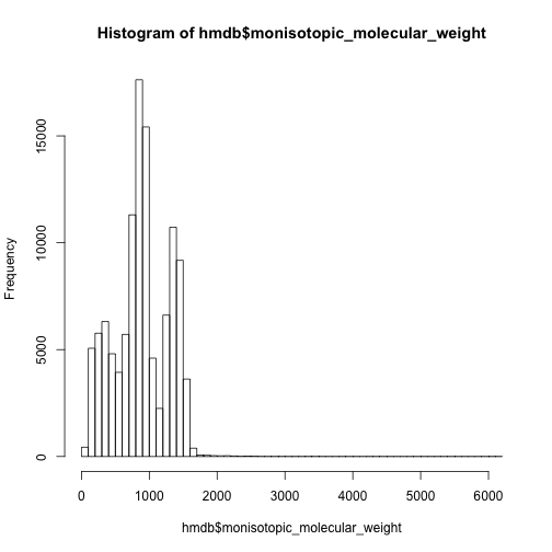
Mass distribution
The mass distribution of all the metabolites is quite different from comment mass spectrum database.
hist(hmdb$monisotopic_molecular_weight,breaks = 50)
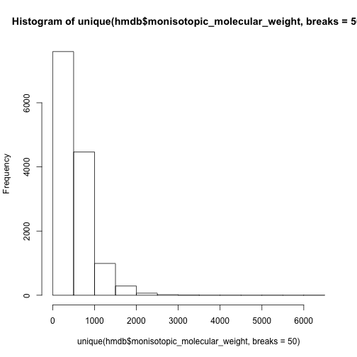
hist(unique(hmdb$monisotopic_molecular_weight,breaks = 50))
However, we could separate the data set into lipid group and other compounds and check again.
lipid <- hmdb[hmdb$super_class == 'Lipids and lipid-like molecules',]
other <- hmdb[!hmdb$super_class == 'Lipids and lipid-like molecules',]
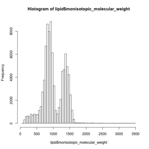
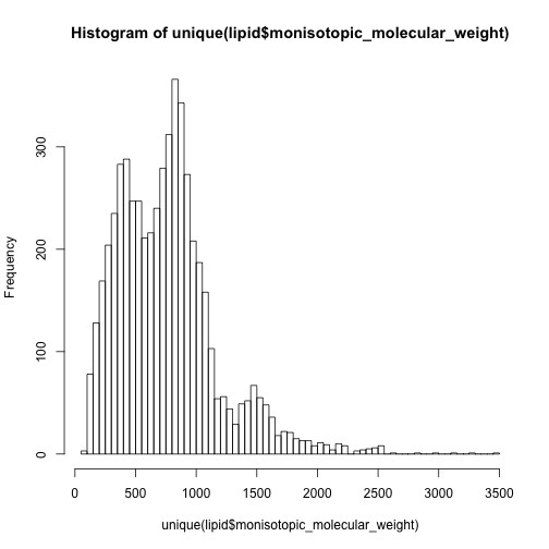
91391 compounds are classified into Lipids and lipid-like molecules and dominate 80% of the metabolites in HMDB database. Their mass distribution is here:
hist(lipid$monisotopic_molecular_weight,breaks = 50)
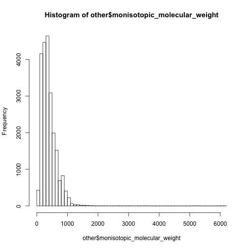
hist(other$monisotopic_molecular_weight,breaks = 50)
hist(unique(lipid$monisotopic_molecular_weight),breaks = 50)
hist(unique(other$monisotopic_molecular_weight),breaks = 50)
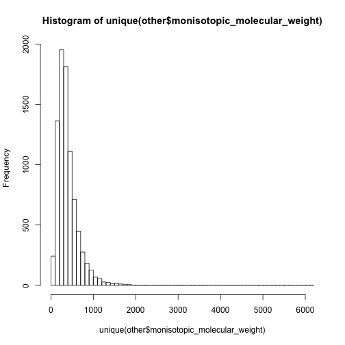
In this case, I have to say the 0-500 are mainly non-lipid metabolites while 500-1000 are dominated by lipids.
Mass defect analysis
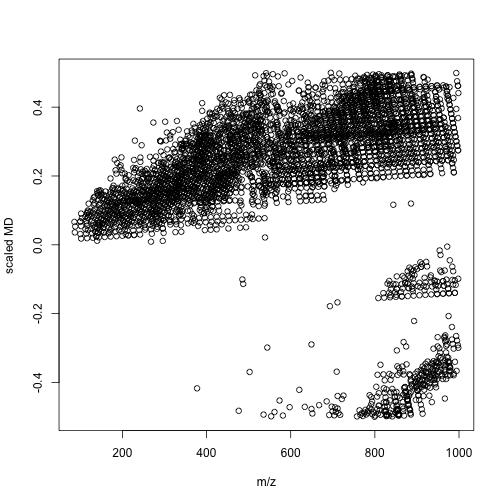
For lipid compounds, we expected a mass defect with certain pattern. Here we use -CH2- as an example.
# lipid
mdalipid <- enviGCMS::getmassdefect(unique(lipid$monisotopic_molecular_weight)[unique(lipid$monisotopic_molecular_weight)<1000],0.9988)
# other
mdaother <- enviGCMS::getmassdefect(unique(other$monisotopic_molecular_weight)[unique(other$monisotopic_molecular_weight)<1000],0.9988)
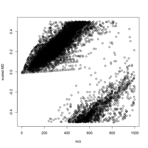
We could find the distribution of mass defect and m/z show different profiles between lipid metabolites and other metabolites. We could use more units to build a model between compounds' class and multiple mass defects. In this case, we might spread one-dimension of data(m/z) into multiple divisions. Then a simple machine learning could give us the answers. I think such way would be a better option compared with build models with thousands of molecular descriptors. When you detected your signal, you know nothing about the structures and such QSPR model would only be useful when you have few candidates.
Home message
-
If you don’t perform lipidomics, MS would be enough for annotation. Of course, you still need high resolution.
-
By using multiple mass defect analysis, we might build a model to class unknown compounds.