In non-targeted metabolomics or environmental non-targeted analysis, throughput is a key factor involving data quality. Typically, we use the same chromatography-mass spectrometry method to run a sample sequence. The sequence executes sample analysis tasks sequentially, meaning the next sample is injected only after the previous one has completely finished running, with each sample generating a single data file. In this process, even if we compress the chromatographic separation time to 15 minutes, we can run fewer than one hundred samples a day at maximum capacity. When considering the quality control (QC) samples included in the injection sequence, the actual number of samples that can be analyzed is even smaller. If thousands of samples need to be processed, the analysis can easily stretch over a month. An instrument running continuously for a year without maintenance can only handle less than ten thousand actual samples, not to mention that each sample might need to be run on different chromatography columns and in both positive and negative ion modes. Under this technical limitation, it is difficult for non-targeted metabolomics or environmental non-targeted analysis to match the throughput of other omics fields, which can handle thousands or tens of thousands of samples per day. Furthermore, as the number of samples increases, batch effects or instrument stability require additional correction, making data quality control exceedingly complex—a true bottleneck issue.
The biggest limitation here is actually sequential injection, where each additional sample adds a full chromatographic separation time. From a data perspective, each sample corresponds to an independent data file, which actually wastes data storage space. For example, when you look at the mass spectrum of sample A eluting at 10 minutes, this spectrum only contains substances from sample A, and most of the space in a full scan is just noise. We can then consider increasing the amount of information by adding more samples while keeping the data space for each sample constant. In simple terms, we don’t wait for one sample to completely finish before injecting the next. Instead, we continuously inject different samples at a fixed time interval, for example, every 1 minute. This way, the data collected at the 10-minute mark of the run will contain substances from sample A separated for 10 minutes, substances from sample B separated for 9 minutes, substances from sample C separated for 8 minutes, and so on. The figure below is an example. The first 10 minutes show the complete separation of 10 substances. What follows is the data that appears when 9 identical samples are injected at one-minute intervals. To the left of the red dashed line is conventional injection, where the mass-to-charge ratio vs. retention time data space is sparse and not utilized efficiently. However, with fixed-interval injections as shown on the right, we can see that the data storage space utilization is significantly improved.
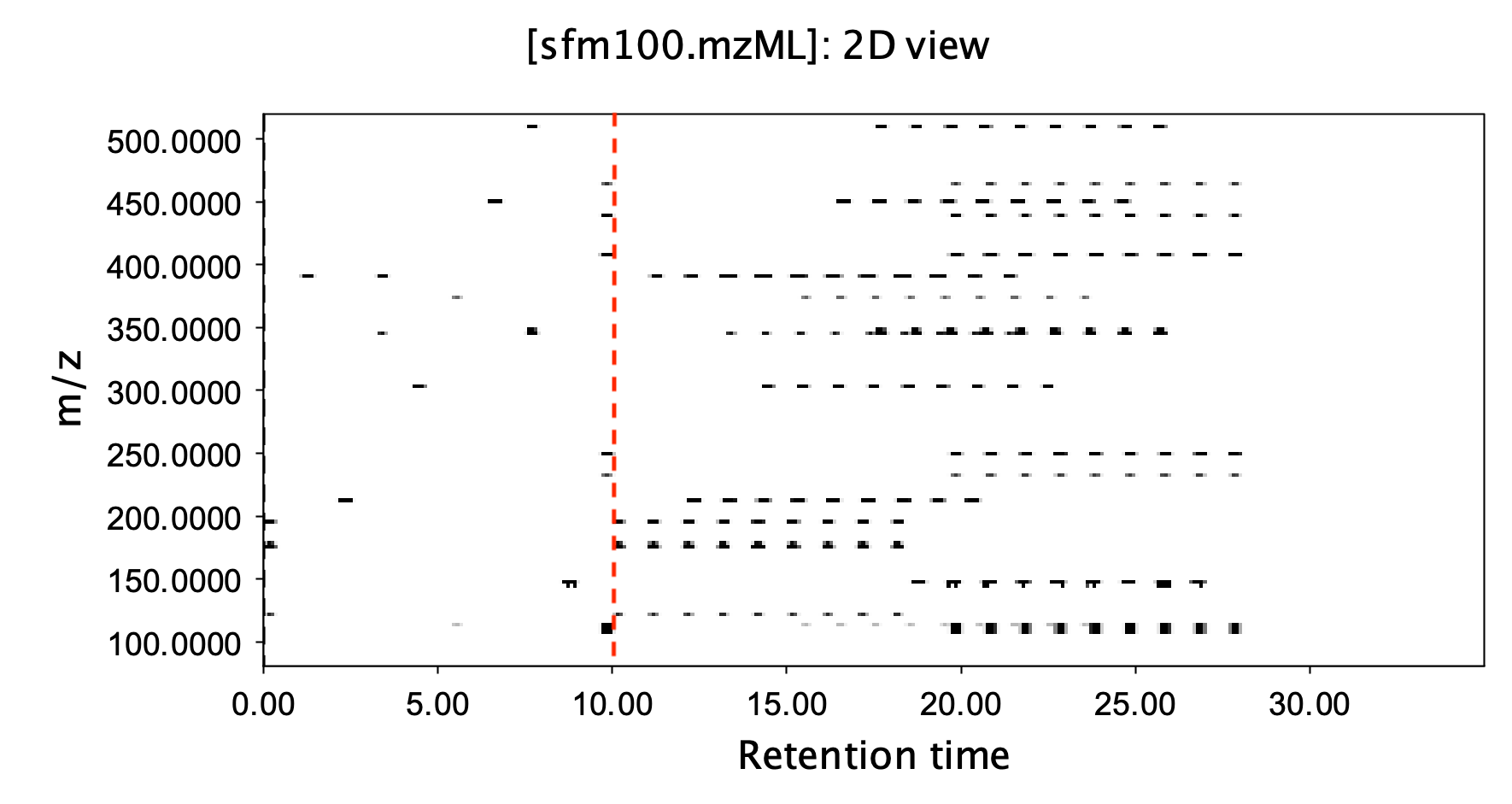
If the chromatographic column’s separation performance is reliable, then theoretically, isomers eluting at different retention times will only interfere with other samples if their time interval is exactly one minute. In this scenario, the marginal time required for each additional sample is theoretically only one minute. This allows us to achieve the analysis of thousands of samples per day. At the same time, the interference from the background or matrix is naturally shortened, mobile phase consumption is greatly reduced, and under isocratic elution, complex peak alignment steps are largely unnecessary. It could be said that in the world of techniques, speed conquers all.
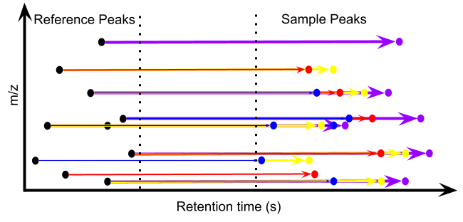
This idea did not come from nowhere. In fact, flow injection technology emerged in the 1970s to increase throughput. Later, with the development of chromatographic technology, methods involving fixed-time-interval injection with isocratic elution also appeared. However, these methods were not for analyzing unknown compounds but for known ones, such as in high-throughput drug screening. If you already know the retention time of a substance, you can find the peak position for the next sample by simply adding the retention time to the injection interval. But what if you don’t know what you are measuring? This brings us back to the previously mentioned scenario. I can inject samples this way, but how do I process the data? As shown in the figure below, the data we collect is like the superimposed image on the left, and we need to recover the individual images on the right.

I submitted an abstract on this topic to this year’s American Society for Mass Spectrometry (ASMS) conference, primarily to solve this problem, and recently submitted a preprint to make this technology public. The solution is quite simple. While we indeed don’t know what we are measuring, we don’t necessarily need to. The most crucial piece of information is that a specific mass-to-charge ratio will appear at a specific retention time. We can obtain this information by running a complete separation of a pooled sample before conducting the fixed-interval injections. Then, we just need to get all the combinations of retention times and mass-to-charge ratios that appear in the pooled sample. Subsequently, the information for a given substance in different samples can be obtained by looking for the response of that mass-to-charge ratio at the expected peak time, which is calculated as its original retention time plus the product of the fixed time interval and the sample injection number. This is like fishing: we don’t know where the fish will appear, but if we have baited a spot beforehand, we can find the corresponding fish by casting our line near that spot. Therefore, this strategy can be understood as “baiting the spot before fishing,” or “Fishing-style Injection.” Note that this method does not require finding a peak for the substance in every sample; it only provides a spatial range to look for the peak. If no peak is found, it means the corresponding sample does not contain that substance. The figure below is a demonstration of the algorithm: the retention time of peak A in the pooled sample, plus the fixed time interval multiplied by (injection number - 1), plus the full separation time of the QC sample, equals the retention time of peak A in the sample with that injection number.
An idea without action is cheap. I noted this idea in my notebook back in 2017, but at the time, I lacked the ability and resources to turn it into action. My current work allows for free exploration, so I revisited this idea and validated it through collaboration in the lab. The most critical part of the practical implementation is to decouple the communication between the chromatography injection and the mass spectrometry acquisition, allowing them to operate independently according to a pre-designed injection sequence without interrupting the MS data collection.
We tested the performance of Fishing-style Injection on two chromatography columns in both positive and negative ion modes. We injected 158 samples in each mode, including a pooled sample as a QC every ten samples, with the total injection time controlled to under six hours. A conventional injection approach would have required several days and a multi-batch design. Because the marginal time added for each additional sample in this method is equal to the fixed time interval (one minute), it is possible to analyze one thousand samples a day while ensuring each sample has 10 minutes of separation time. Repeated tests showed that the retention time shift was within 10 seconds; the reversed-phase column actually performed better, and the shift on the HILIC column was also within an acceptable range. In terms of quantitative performance, within the 10-minute isocratic elution window, although we found 1000-3000 peaks during the “baiting” process, after considering only the peaks with a response deviation of less than 30% in the intra-sequence pooled samples and removing peaks found in the blank, we could still obtain 450-738 stable peaks. Again, the reversed-phase column performed better than the HILIC column. This result is already in the same order of magnitude as the number of peaks obtained with gradient injection after applying similar quality control standards. Furthermore, the issue of isomeric interference mentioned earlier does exist, but for blood metabolomics specifically, fewer than 2% of the peaks were affected. If you are analyzing lipids, you should definitely evaluate this effect first and optimize for a fixed interval time that minimizes interference. If throughput is a priority and you have tested that the compounds you care about can be separated by the column, then Fishing-style Injection offers a natural advantage in speed and cost. The cost per sample can be controlled to under $10, which is at least an order of magnitude lower than current injection methods, making high-throughput mass spectrometry screening a reality. Moreover, I have already written an open-source software package for the most critical data processing part of this method. If you want to try this method, there is no need for physical modifications to your existing instrument; you just need to control the chromatography injection and data acquisition separately. In fact, the mobile phase can be switched to gradient elution, but the injection interval would no longer be fixed and would need to be optimized for the column. Alternatively, the interval could be kept fixed, but the algorithm would need to recognize the elution pattern. I will leave these parts for future improvements by others.
Feel free to try it out!
Preprint link: https://chemrxiv.org/engage/chemrxiv/article-details/6897568d728bf9025ec3ab62