In mass spectrometry based untargeted analysis, raw data from instrument contain peaks level information. However, we actually care about compounds level information. For target analysis, quantitative and qualitative ions could stand for the target compounds. However, in untargeted analysis, full scan mode will collect all the charged compounds’ ions. One compound could generate multiple ions such as adducts, neutral loss, multiple charged ions, isotopougue and/or fragmental ions and those peaks are highly correlated with each other. If we will perform the statistical analysis at compounds level, those highly correlated ions will disturb the independent assumption of those statistical analysis. In this case, we need algorithm to remove such redundant peaks or select pseudo targeted ions for unknown compounds. Ideally, selection of molecular ion will make the following analysis much easier.
To detect such redundant peaks, two relationships could be used: paired mass distance (PMD) and paired correlation. I developed GlobalStd algorithm to remove such redundant peaks based on PMD relationship. However, I actually added the function to use correlation along with PMD in this algorithm. To make the details clear, I also added functions to extract independent peaks based on correlation, as well as the ions clusters extraction function. The ions clusters could be treated the pseudo spectra detection algorithm. In this case, we could not only extract the independent ions for compounds level analysis, but also grab the pseudo specturm of this compounds for annotation purpose.
Here I will demo how to perform such analysis based on PMD package:
# use dev version of PMD package
# remotes::install_github('yufree/pmd')
library(pmd)
library(enviGCMS)
# load demo data
data(spmeinvivo)
# perform GlobalStd algorithm
list <- globalstd(spmeinvivo)
## 75 retention time cluster found.## 380 paired masses found## 9 unique within RT clusters high frequency PMD(s) used for further investigation.## 719 isotopologue(s) related paired mass found.## 492 multi-charger(s) related paired mass found.## 8 retention group(s) have single peaks. 14 23 32 33 54 55 56 75## 11 group(s) with multiple peaks while no isotope/paired relationship 4 5 7 8 11 41 42 49 68 72 73## 9 group(s) with multiple peaks with isotope without paired relationship 2 9 22 26 52 62 64 66 70## 4 group(s) with paired relationship without isotope 1 10 15 18## 43 group(s) with paired relationship and isotope 3 6 12 13 16 17 19 20 21 24 25 27 28 29 30 31 34 35 36 37 38 39 40 43 44 45 46 47 48 50 51 53 57 58 59 60 61 63 65 67 69 71 74## 297 std mass found.## PMD frequency cutoff is 6 by PMD network analysis with largest network average distance 5.99 .## 57 groups were found as high frequency PMD group.## 0 was found as high frequency PMD.
## 1.98 was found as high frequency PMD.
## 2.01 was found as high frequency PMD.
## 2.02 was found as high frequency PMD.
## 6.97 was found as high frequency PMD.
## 11.96 was found as high frequency PMD.
## 12 was found as high frequency PMD.
## 12.04 was found as high frequency PMD.
## 13.98 was found as high frequency PMD.
## 14.02 was found as high frequency PMD.
## 14.05 was found as high frequency PMD.
## 15.99 was found as high frequency PMD.
## 16.03 was found as high frequency PMD.
## 19.04 was found as high frequency PMD.
## 28.03 was found as high frequency PMD.
## 30.05 was found as high frequency PMD.
## 31.99 was found as high frequency PMD.
## 37.02 was found as high frequency PMD.
## 42.05 was found as high frequency PMD.
## 48.04 was found as high frequency PMD.
## 48.98 was found as high frequency PMD.
## 49.02 was found as high frequency PMD.
## 54.05 was found as high frequency PMD.
## 56.06 was found as high frequency PMD.
## 56.1 was found as high frequency PMD.
## 58.04 was found as high frequency PMD.
## 58.08 was found as high frequency PMD.
## 58.11 was found as high frequency PMD.
## 63.96 was found as high frequency PMD.
## 66.05 was found as high frequency PMD.
## 68.06 was found as high frequency PMD.
## 70.04 was found as high frequency PMD.
## 70.08 was found as high frequency PMD.
## 74.02 was found as high frequency PMD.
## 80.03 was found as high frequency PMD.
## 82.08 was found as high frequency PMD.
## 88.05 was found as high frequency PMD.
## 91.1 was found as high frequency PMD.
## 93.12 was found as high frequency PMD.
## 96.09 was found as high frequency PMD.
## 101.05 was found as high frequency PMD.
## 108.13 was found as high frequency PMD.
## 110.11 was found as high frequency PMD.
## 112.16 was found as high frequency PMD.
## 116.08 was found as high frequency PMD.
## 122.15 was found as high frequency PMD.
## 124.16 was found as high frequency PMD.
## 126.14 was found as high frequency PMD.
## 148.04 was found as high frequency PMD.
## 150.2 was found as high frequency PMD.
## 173.18 was found as high frequency PMD.
## 191.08 was found as high frequency PMD.
## 191.15 was found as high frequency PMD.
## 192.19 was found as high frequency PMD.
## 194.2 was found as high frequency PMD.
## 267.25 was found as high frequency PMD.
## 325.3 was found as high frequency PMD.# get new list with independent peaks
listi <- getfilter(list,rowindex = list$stdmassindex)Here we have 297 peaks compared with original 1459 peaks. If we removed the right redundant peaks, the PCA score plot will not change too much with a much smaller data set.
# plot the comparision
par(mfrow = c(1,2),mar = c(4,4,2,1)+0.1)
plotpca(list$data,lv = as.numeric(as.factor(list$group)),main = "all peaks")
plotpca(listi$data,lv = as.numeric(as.factor(listi$group)),main = " independent peaks")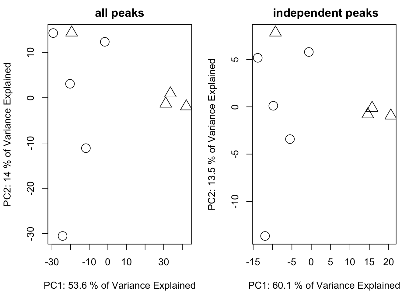
The GlobalStd algorithm with default setting will not use intensity data. However, if we could use intensity data to refine the result, we could select the base peaks of each pseudo spectrum. After consideration of correlation relationship, we could further select the base independent peaks.
base <- getcluster(list)
# get the new list with independent base peaks
listb <- getfilter(list,rowindex = base$stdmassindex2)
# get the new list with reduced independent base peaks
basei <- getcluster(list,corcutoff = 0.9)
listib <- getfilter(list,rowindex = basei$stdmassindex2)
If we didn’t use PMD, we could also detect the correlation cluster within narrow retention time window as pseudo spectra. I also supplied function to select the correlation independent peaks and base correlation independent peaks.
ci <- getcorcluster(spmeinvivo)## 75 retention time cluster found.# get the new list with correlation independent peaks
listci <- getfilter(list,rowindex = ci$stdmassindex)
# get the new list with base correlation independent peaks
listcib <- getfilter(list,rowindex = ci$stdmassindex2)We could compare the compare reduced result using PCA similarity factor. A good peak selection algorithm could show a high PCA similarity factor compared with original data set while retain the minmized number of peaks.
par(mfrow = c(2,3),mar = c(4,4,2,1)+0.1)
plotpca(listi$data,lv = as.numeric(as.factor(list$group)),main = paste(sum(list$stdmassindex),"independent peaks"))
plotpca(listb$data,lv = as.numeric(as.factor(list$group)),main = paste(sum(base$stdmassindex2),"independent base peaks"))
plotpca(listib$data,lv = as.numeric(as.factor(list$group)),main = paste(sum(basei$stdmassindex2),"reduced independent base peaks"))
plotpca(listci$data,lv = as.numeric(as.factor(list$group)),main = paste(sum(ci$stdmassindex),"peaks without correlationship"))
plotpca(listcib$data,lv = as.numeric(as.factor(list$group)),main = paste(sum(ci$stdmassindex2),"base peaks without correlationship"))
plotpca(list$data,lv = as.numeric(as.factor(list$group)),main = paste(nrow(list$data),"all peaks"))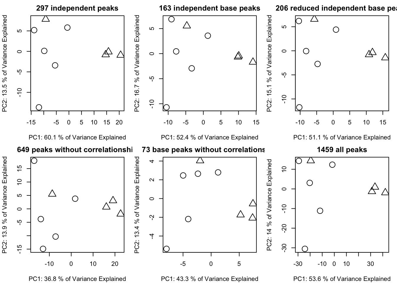
In this case, five peaks selection algorithms are fine to stand for the original peaks. However, the independent base peaks retain the most information with relative low numbers of peaks.