自动化机器学习(AutoML)大概在四五年前非常火,现在基本熄火进入平稳期与实用期了,是时候回顾下了。
首先,自动化机器学习同样是用来做机器学习的,机器学习适合做的领域自动化机器学习都可以做。这里自动化主要是把调参、变量选择、模型选择、模型集成等传统需要机器学习专家来做的事流程化自动化执行,可以算是程序员自掘职业坟墓的又一成果。
现在很多学科都在谈机器学习,有些是当辅助用,有些是当魔法用,还有些单纯用来要饭忽悠人的。但你去看看高校培养计划会发现虽然很多学科前沿展望里都在鼓吹,培养上基本放羊,全靠学生自学。这样的后果就是同样都是自称做机器学习的,有的是调包流,跑个泰坦尼克幸存者就说懂机器学习,满嘴随机森林支持向量机,走个MNIST敢自称会深度学习。另外一些是y=f(x)流,精于把自己学科问题抽象成一个可训练的模型,然后直接找机器学习专家合作,根本不管模型细节;另一些则是解释流,只对线性模型跟决策树感兴趣,别的都不关心。
毫无意外,自动化机器学习最适合的是第二类人,当然他们最好对基础模型本身原理有感知。但真到预测性问题上就无所谓了,表现最好的一般是多个不同模型集成的。从原理上说,集成学习就是尝试组合不同原理或假设的模型来尽量多的攫取数据中跟预测目标相关的信息。从这个角度上看,单纯依赖某一种模型对于结构复杂问题的信息利用效率都很难高到哪去;而现在流行的深度学习基本就是对原始数据进行各种各样的线性或非线性变换组合,旨在通过各种基础模型的变换组合尽量多的捕集数据中的信息;而更进一步说,类似AlphaFold2这种变形金刚结构的深度学习框架则在编码器阶段融入了学科知识,例如蛋白共源性或氨基酸结合的亲和度,这样在解决具体学科问题上同时包含了通用机器学习模型对信息的穷举与专业生物化学知识来辅助训练,达到了很出色的表现。当然,这种专业知识跟机器学习深度融合的模型就不能指望自动化机器学习了,得从模型构架上重新设计,此处人才到今天都是缺的,现有的基本都进了大厂的研究机构。
对于大多数当前的应用水平使用者而言,其实自动化机器学习是非常好用的工具。应用者日常面对的就是具体的科学问题,将其转为一个可训练的模型然后交给自动化机器学习去训练,最后或者预测或者尝试解释,然后把结果有效告知决策者或公众。其实这里面应用者更多是一个翻译角色,把隐藏在数据中有价值的规律或现象用人话或可视化手段表示出来,所以精力更多在沟通而不是具体技术上,大量时间都在洗数据跟出报告。虽然现在很多深度学习模型在某些领域已经可以做到自动抽取特征了,但面对具体的问题,洗出一个跟问题相关的特征数据还是很难被通用技术代劳的,或者说通用技术效率相对低下。举个例子,要预测污水厂效率,有人会把所有工厂传感数据送进模型,而有经验的人可以直接用跟污水处理相关的技术指标,前后训练用的时间完全不同,后者可以达到实时预测。现在很多人转码农经常是直接把自己专业知识给扔了,其实如果利用得当,其职业前景或岗位不可替代性要比搞通用算法那批人好很多。
其实,自动化机器学习另一个相关议题在于迁移学习。也就是说有很多已经训练好的通用模型可以直接调用或在其构架上定向训练。如果是自然语言处理任务,可以用Open AI GPT系列模型,虽然不开源(开源可以用Bert),但通过调用API一样可以用。图像识别可以拿 ResNet 或 VGG16 来用,这里可以省不少事。这些已经训练好的模型都算是大模型,如果想定向优化到一个小数据集或数据领域里可以特异性去训练其中一层或几层,也可以稍微调下构架在后面补上一两个层来收集数据集中信息,鉴于这些都属于深度学习领域,最好还是先去搞明白最近三五年的一些进展再动手。不过实际研究中数据可能既不是图像也不是文字,没有可直接迁移的通用模型,而且数据量也不大,所以不容易受益于机器学习领域的进展。不过鉴于现在自动化机器学习已经涉及了深度学习,所以自动化训练一个模型问题也不大。
从应用角度,自动化机器学习模型很容易构建,基本上你只需要明确目标跟预测变量就可以了。机器学习领域最喜欢折腾的是自然语言跟图片的分类、识别等问题,但应用领域更常见的数据类型是表格或者说样本-特征矩阵,当然有些特征是明确的量化值,有的则可能也是图片、语音等数据。举个例子,我想知道一个人是否得呼吸道疾病,那么我可以收集其流行病学调查问卷数据,也可以收集其体检的胸片,还可以收集其读某段文字的发音数据等。这里任何单一来源数据都可以单独构建一个预测模型,然后你可以做个集成学习;另一个思路则是把每个来源的数据都看成一组特征,将所有特征转化整合在一张数据表里去预测。这里很难说哪种思路效果更好,这里只需要解决非结构化数据(语音、图像、文字等)的特征提取两者在本质上就是一回事了,不过眼下还是要区分下结构化数据跟非结构化数据模型好一些,两者模型构建逻辑上还是区别很大的。
下面我们来个实战,看看这个操作有多简单。这里我用到的是H2O的AutoML这个框架。
# 读取一个代谢组学示例数据,x是所有的特征峰,y是肺癌与否
download.file('https://github.com/yufree/rmwf/raw/master/inst/demodata/untarget/MTBLS28posmzrt.csv','pos.csv')
mzrt <- enviGCMS::getmzrtcsv('pos.csv')
lv <- ifelse(grepl('Control',mzrt$group$sample_group),'control','case')
trainIndex <- sample(1:1005,700)
train <- mzrt$data[, trainIndex]
train <- cbind.data.frame(Y=lv[trainIndex],t(train))
test  <- mzrt$data[,-trainIndex]
test  <- cbind.data.frame(Y=lv[-trainIndex],t(test))
y = 'Y'
pred = setdiff(names(train), y)
#convert variables to factors
train[,y] = as.factor(train[,y])
test[,y] = as.factor(test[,y])
library(h2o)
##
## ----------------------------------------------------------------------
##
## Your next step is to start H2O:
## > h2o.init()
##
## For H2O package documentation, ask for help:
## > ??h2o
##
## After starting H2O, you can use the Web UI at http://localhost:54321
## For more information visit https://docs.h2o.ai
##
## ----------------------------------------------------------------------##
## Attaching package: 'h2o'## The following objects are masked from 'package:stats':
##
## cor, sd, var## The following objects are masked from 'package:base':
##
## &&, %*%, %in%, ||, apply, as.factor, as.numeric, colnames,
## colnames<-, ifelse, is.character, is.factor, is.numeric, log,
## log10, log1p, log2, round, signif, trunch2o.init()## Connection successful!
##
## R is connected to the H2O cluster:
## H2O cluster uptime: 20 minutes 42 seconds
## H2O cluster timezone: America/New_York
## H2O data parsing timezone: UTC
## H2O cluster version: 3.36.1.2
## H2O cluster version age: 1 month and 28 days
## H2O cluster name: H2O_started_from_R_yufree_stx351
## H2O cluster total nodes: 1
## H2O cluster total memory: 3.76 GB
## H2O cluster total cores: 8
## H2O cluster allowed cores: 8
## H2O cluster healthy: TRUE
## H2O Connection ip: localhost
## H2O Connection port: 54321
## H2O Connection proxy: NA
## H2O Internal Security: FALSE
## R Version: R version 4.2.0 (2022-04-22)train_h = as.h2o(train)##
|
| | 0%
|
|======================================================================| 100%test_h = as.h2o(test)##
|
| | 0%
|
|======================================================================| 100%# Run AutoML for 20 base models
aml = h2o.automl(x = pred, y = y,
training_frame = train_h,
max_models = 10,
seed = 42
)##
|
| | 0%
## 15:55:44.94: AutoML: XGBoost is not available; skipping it.
|
| | 1%
|
|= | 1%
|
|= | 2%
|
|== | 2%
|
|== | 3%
|
|=== | 4%
|
|==== | 5%
|
|==== | 6%
|
|===== | 7%
|
|===== | 8%
|
|====== | 9%
|
|======= | 10%
|
|======== | 11%
|
|======== | 12%
|
|========= | 13%
|
|========== | 14%
|
|========== | 15%
|
|=========== | 16%
|
|============ | 17%
|
|============ | 18%
|
|============= | 19%
|
|============== | 20%
|
|============== | 21%
|
|=============== | 21%
|
|=============== | 22%
|
|================ | 23%
|
|================ | 24%
|
|================== | 25%
|
|=================== | 26%
|
|======================================================================| 100%# AutoML Leaderboard
lb <- h2o.get_leaderboard(object = aml, extra_columns = "ALL")
lb## model_id auc logloss aucpr
## 1 StackedEnsemble_BestOfFamily_1_AutoML_2_20220724_155544 0.8310 0.4942 0.8296
## 2 StackedEnsemble_AllModels_1_AutoML_2_20220724_155544 0.8264 0.5008 0.8267
## 3 GBM_1_AutoML_2_20220724_155544 0.8182 0.5191 0.8182
## 4 GBM_4_AutoML_2_20220724_155544 0.8135 0.5224 0.8197
## 5 GLM_1_AutoML_2_20220724_155544 0.8106 0.5310 0.7991
## 6 GBM_2_AutoML_2_20220724_155544 0.8063 0.5304 0.8081
## mean_per_class_error rmse mse training_time_ms predict_time_per_row_ms
## 1 0.2450 0.4044 0.1635 547 0.04390
## 2 0.2544 0.4069 0.1656 655 0.03897
## 3 0.2843 0.4146 0.1719 1244 0.01945
## 4 0.2677 0.4170 0.1739 2936 0.01449
## 5 0.3011 0.4181 0.1748 5889 0.01053
## 6 0.2782 0.4201 0.1765 2170 0.01257
## algo
## 1 StackedEnsemble
## 2 StackedEnsemble
## 3 GBM
## 4 GBM
## 5 GLM
## 6 GBM
##
## [12 rows x 10 columns]# prediction
pred <- h2o.predict(aml,test_h[,-1])##
|
| | 0%
|
|======================================================================| 100%caret::confusionMatrix(test$Y, as.data.frame(pred)$predict)## Confusion Matrix and Statistics
##
## Reference
## Prediction case control
## case 99 51
## control 18 137
##
## Accuracy : 0.774
## 95% CI : (0.723, 0.82)
## No Information Rate : 0.616
## P-Value [Acc > NIR] : 3.33e-09
##
## Kappa : 0.546
##
## Mcnemar's Test P-Value : 0.000117
##
## Sensitivity : 0.846
## Specificity : 0.729
## Pos Pred Value : 0.660
## Neg Pred Value : 0.884
## Prevalence : 0.384
## Detection Rate : 0.325
## Detection Prevalence : 0.492
## Balanced Accuracy : 0.787
##
## 'Positive' Class : case
## # explain the model
h2o.explain(aml, test_h)##
##
## Leaderboard
## ===========
##
## > Leaderboard shows models with their metrics. When provided with H2OAutoML object, the leaderboard shows 5-fold cross-validated metrics by default (depending on the H2OAutoML settings), otherwise it shows metrics computed on the newdata. At most 20 models are shown by default.
##
##
## | | model_id | auc | logloss | aucpr | mean_per_class_error | rmse | mse | training_time_ms | predict_time_per_row_ms | algo
## |:---:|:---:|:---:|:---:|:---:|:---:|:---:|:---:|:---:|:---:|:---:|
## | **1** |StackedEnsemble_BestOfFamily_1_AutoML_2_20220724_155544 | 0.831017204354158 | 0.49423273504537 | 0.82957926642421 | 0.245028344811131 | 0.404395617724151 | 0.163535815634498 | 547 | 0.043897 | StackedEnsemble |
## | **2** |StackedEnsemble_AllModels_1_AutoML_2_20220724_155544 | 0.826364376866685 | 0.500763642152662 | 0.826674410682095 | 0.254395708373444 | 0.406881363235919 | 0.16555244374872 | 655 | 0.038967 | StackedEnsemble |
## | **3** |GBM_1_AutoML_2_20220724_155544 | 0.818198273805116 | 0.519098325610369 | 0.818161321019998 | 0.284320259340623 | 0.414569323179071 | 0.171867723721153 | 1244 | 0.019452 | GBM |
## | **4** |GBM_4_AutoML_2_20220724_155544 | 0.813463168201153 | 0.522399583342484 | 0.819736816333827 | 0.267700079809773 | 0.416972629142305 | 0.173866173453847 | 2936 | 0.014492 | GBM |
## | **5** |GLM_1_AutoML_2_20220724_155544 | 0.810628687088095 | 0.530963098927506 | 0.799140535379632 | 0.301088539481154 | 0.418120234490234 | 0.174824530490168 | 5889 | 0.010533 | GLM |
## | **6** |GBM_2_AutoML_2_20220724_155544 | 0.806292630349106 | 0.530399779705598 | 0.808097284982117 | 0.278198767473815 | 0.420108424358518 | 0.176491088216996 | 2170 | 0.012573 | GBM |
## | **7** |GBM_5_AutoML_2_20220724_155544 | 0.803375871119558 | 0.53609778763023 | 0.80905995260343 | 0.255708044331449 | 0.421280326474034 | 0.177477113474069 | 2286 | 0.012849 | GBM |
## | **8** |GBM_3_AutoML_2_20220724_155544 | 0.801232526185011 | 0.539889449123235 | 0.808464403923565 | 0.266243757147911 | 0.424605908974098 | 0.18029017793572 | 2338 | 0.012583 | GBM |
## | **9** |GBM_grid_1_AutoML_2_20220724_155544_model_1 | 0.78743859995557 | 0.553638512512293 | 0.794143332750029 | 0.296242358419931 | 0.431314041585845 | 0.186031802469116 | 2419 | 0.012655 | GBM |
## | **10** |DRF_1_AutoML_2_20220724_155544 | 0.785599684052033 | 0.568249606521988 | 0.79898788403003 | 0.333711812669184 | 0.438422374043897 | 0.192214178062287 | 1056 | 0.013243 | DRF |
## | **11** |XRT_1_AutoML_2_20220724_155544 | 0.75527608421988 | 0.590779332812731 | 0.756576018081061 | 0.30185783987033 | 0.449392172222291 | 0.20195332445467 | 862 | 0.01249 | DRF |
## | **12** |DeepLearning_1_AutoML_2_20220724_155544 | 0.642542722911987 | 0.765522963151034 | 0.664741919283686 | 0.426007289841121 | 0.509052417909465 | 0.259134364179472 | 315 | 0.015305 | DeepLearning |
##
##
## Confusion Matrix
## ================
##
## > Confusion matrix shows a predicted class vs an actual class.
##
##
##
## StackedEnsemble_BestOfFamily_1_AutoML_2_20220724_155544
## -------------------------------------------------------
##
## | | case | control | Error | Rate
## |:---:|:---:|:---:|:---:|:---:|
## | **case** |113 | 37 | 0.246666666666667 | =37/150 |
## | **control** |23 | 132 | 0.148387096774194 | =23/155 |
## | **Totals** |136 | 169 | 0.19672131147541 | =60/305 |
##
##
## Variable Importance
## ===================
##
## > The variable importance plot shows the relative importance of the most important variables in the model.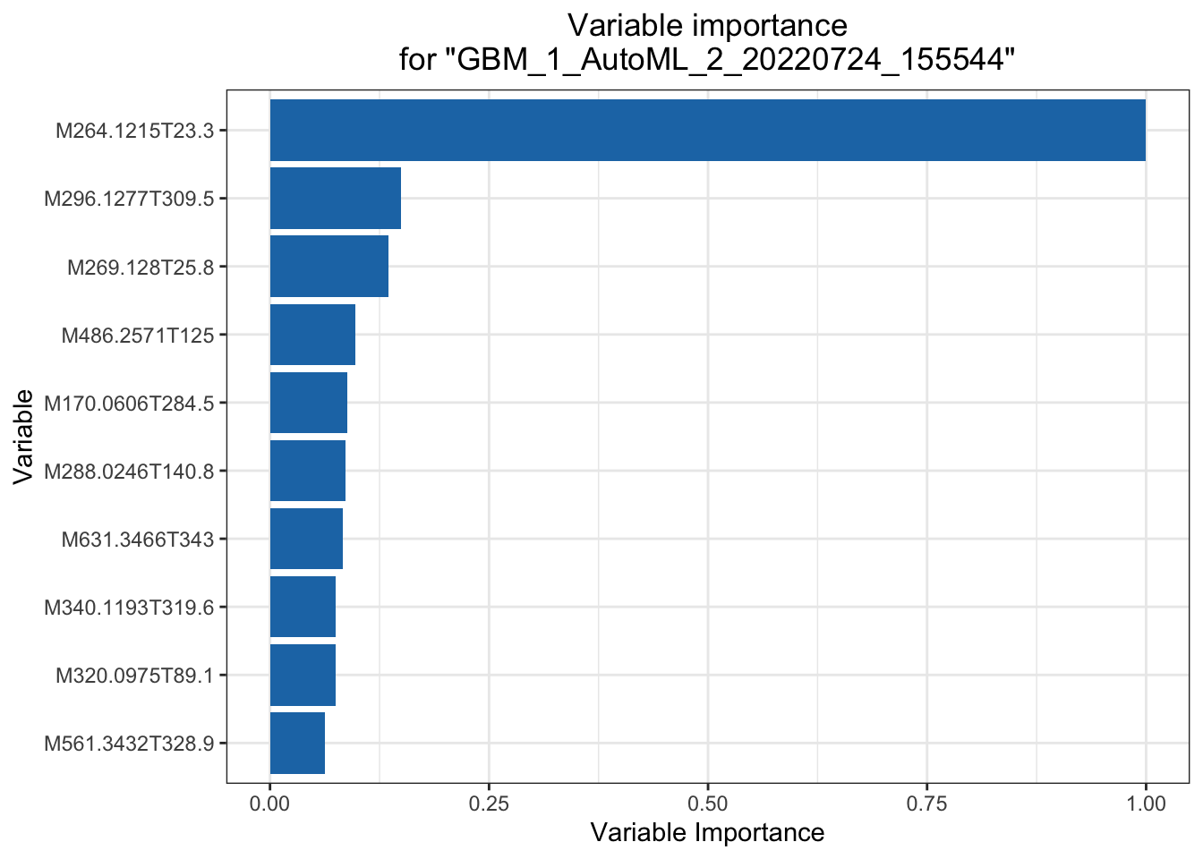
##
##
## Variable Importance Heatmap
## ===========================
##
## > Variable importance heatmap shows variable importance across multiple models. Some models in H2O return variable importance for one-hot (binary indicator) encoded versions of categorical columns (e.g. Deep Learning, XGBoost). In order for the variable importance of categorical columns to be compared across all model types we compute a summarization of the the variable importance across all one-hot encoded features and return a single variable importance for the original categorical feature. By default, the models and variables are ordered by their similarity.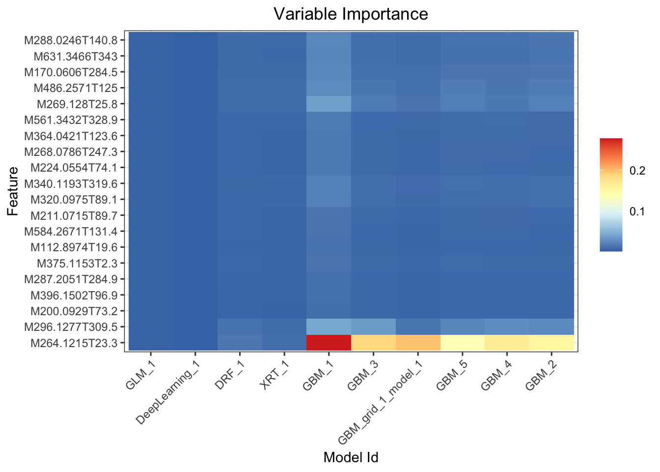
##
##
## Model Correlation
## =================
##
## > This plot shows the correlation between the predictions of the models. For classification, frequency of identical predictions is used. By default, models are ordered by their similarity (as computed by hierarchical clustering).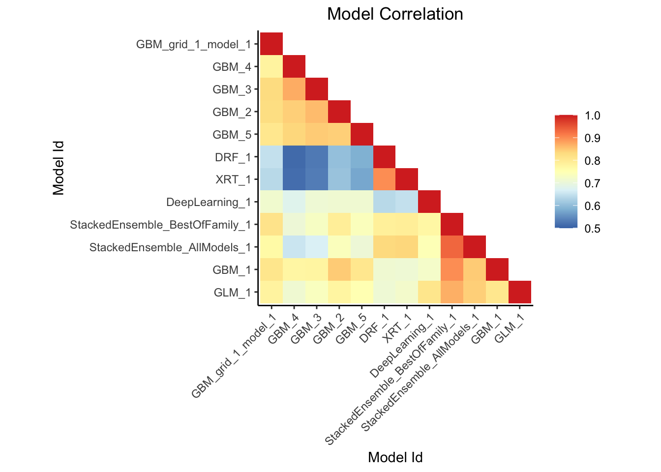
## Interpretable models: GLM_1_AutoML_2_20220724_155544
##
##
## SHAP Summary
## ============
##
## > SHAP summary plot shows the contribution of the features for each instance (row of data). The sum of the feature contributions and the bias term is equal to the raw prediction of the model, i.e., prediction before applying inverse link function.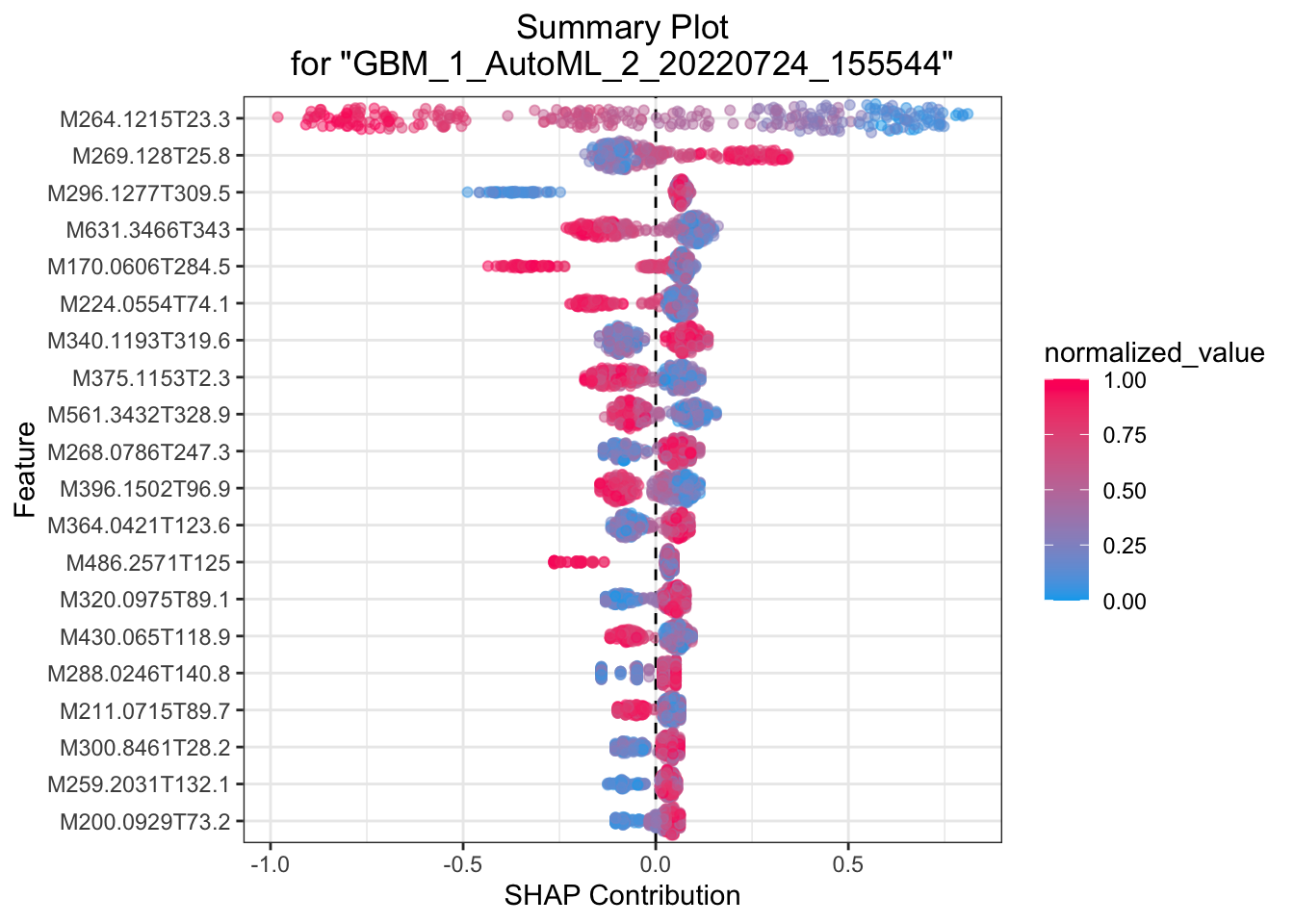
##
##
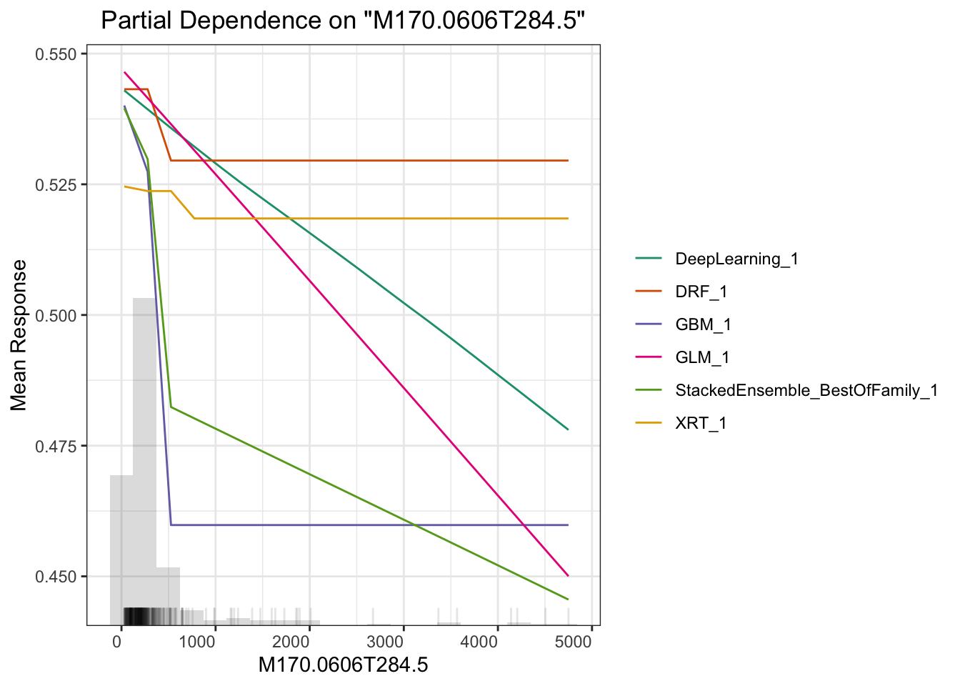
## Partial Dependence Plots
## ========================
##
## > Partial dependence plot (PDP) gives a graphical depiction of the marginal effect of a variable on the response. The effect of a variable is measured in change in the mean response. PDP assumes independence between the feature for which is the PDP computed and the rest.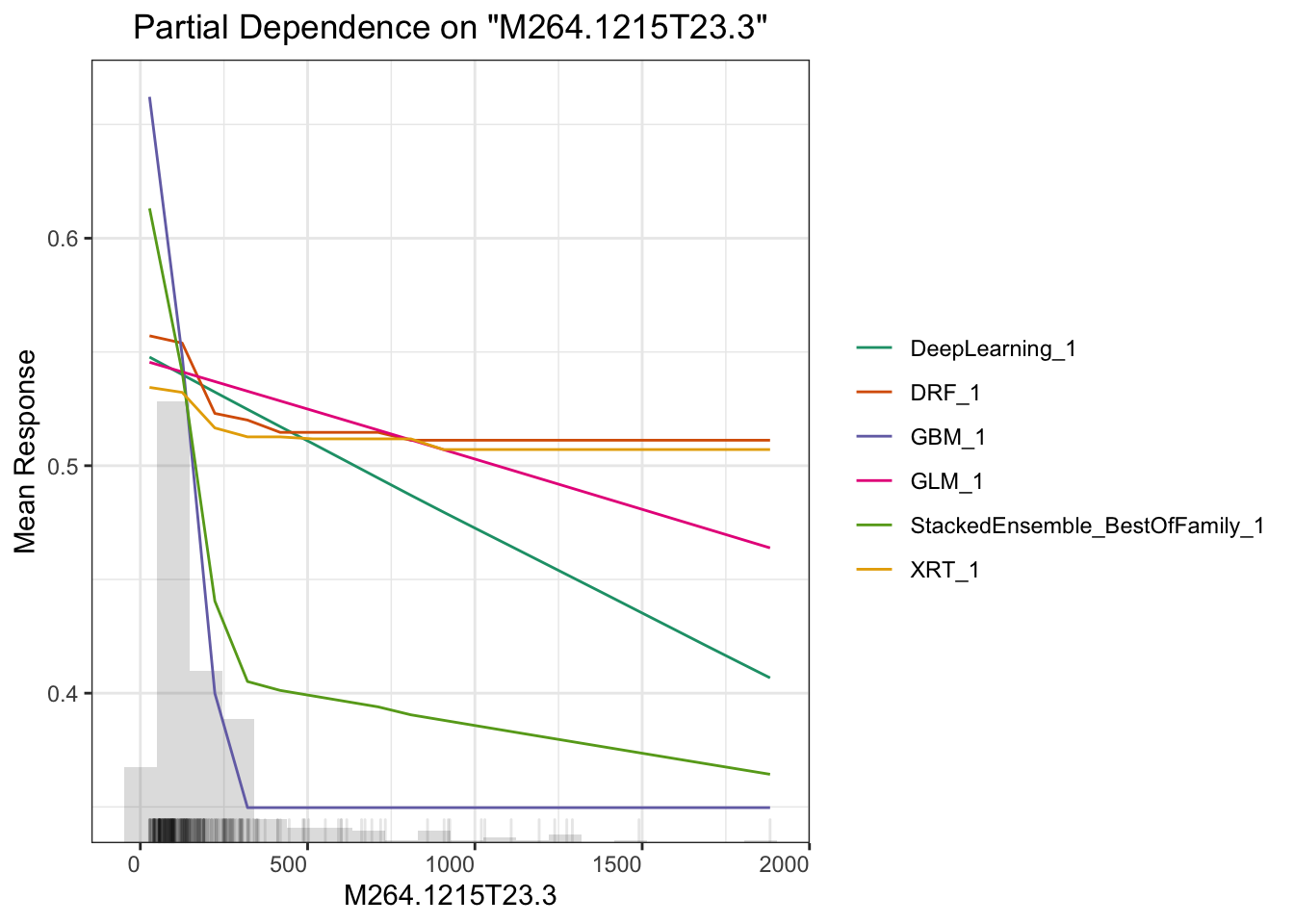
# plot M264.1215T23.3
boxplot(test$M264.1215T23.3~test$Y,xlab='',ylab='response')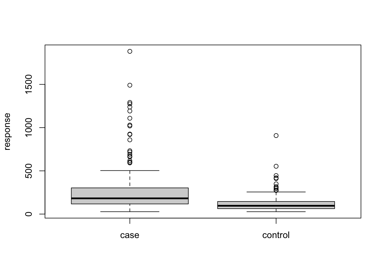
h2o.shutdown(prompt = F)从上面例子可以看出,一个完整的自动化机器学习要包括下面几个步骤:
- 读入数据并至少拆分为训练集与检验集
- 在训练集上进行自动化机器学习
- 检查预测模型的表现
- 在检验集上观察预测效果
- 解释模型
这里我们观察到检验集上模型表现弱于训练集,存在过拟合,可考虑调整下交叉检验的参数。当然现在自动训练的模型表现比我一年多前用随机森林做同样数据的演示效果还差一点,但差距并不大可接受。关键在于上面那段代码的可移植性要比单纯针对某个模型要好很多,科研中引入机器学习更多是做探索,有段随时可测的代码会让整个流程更顺畅。
这里另一个相关主题是可解释性机器学习。我们做研究的预测率高几个百分点意义不大,但要是能说出哪个变量对预测的贡献高低并展示出来就很有意义了。这方面全局影响可以用Partial Dependence Plot(PDP) 来表示,或者给出变量重要性,或者给出 SHAP 贡献值,这里面 PDP 是针对全局预测的,还有些其他的例如 LIME 可以对单一预测给出变量重要性,具体怎么用需要结合你的科学问题来探索。
总之,我认为当前自动化机器学习对实际科研问题已经是一种可以用的水平了,可以快速试错一些想法找一些方向。当然,你最好是明白自己在干什么。